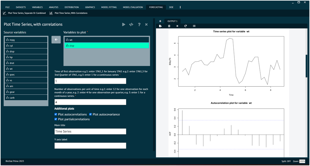
Plot Time Series with Correlations
When dealing with time series forecasting, the concept of correlation can be relevant, particularly in cases where there are multiple time series, and user want to understand the relationships between them. Correlation measures the strength and direction of a linear relationship between two variables. Correlation analysis can guide the selection of variables for inclusion in forecasting models. Variables with strong correlations might have predictive power and contribute to the accuracy of the model.
Creates time series plot with autocorrelations, autocovariance and partial correlations.
To analyse it in BioStat Prime user must follow the steps as given.
- Steps
Load the dataset -> Click on the Forecasting tab in main menu -> Select Plot Time Series With Correlations -> Choose variables to plot -> Write Time of first observation -> Write Number of observations per unit of time -> Execute.

Arguments
- vars
selected variables to plot
- start
Time of first observation should be entered in the format year,month or year,quarter e.g.( if your data is organized in months the 1992,1 for Jan 1992 or if your data is organized in quarters then 1992,1 refers to the first quarter of 1992.
- frequency
Number of observations in unit time. Example: for monthly there are 12 observation in a year. For quarterly there are 4 observation in a year.
- autocorrelation
if TRUE an autocorrelation plot will also be generated.
- autocovariance
if TRUE an autocovariance plot will also be generated.
- partialautocorrelations
if TRUE an partial autocorrelations plot will also be generated.
- plot.type
"multiple" for separate and "single" for combined plot.
- main
main title of the plot
- ylab
title for the y axis
- dataset
the name of the dataset from which the vars has been picked.