Ordinal Regression
This function fits a logistic or probit regression model to an ordered factor response. The default logistic case is proportional odds logistic regression, after which the function is named.
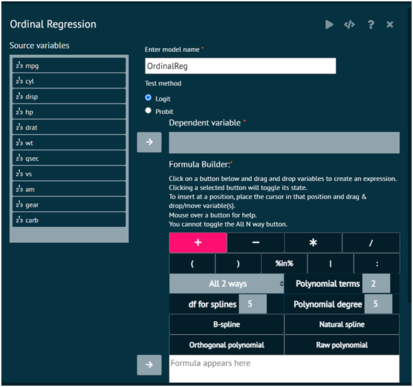
To analyse it in BioStat Prime user must follow the steps as given.
- Steps
Load the dataset -> Click on the Model Fitting tab in main menu -> Select Regression -> This leads to analysis techniques, choose Ordinal Regression -> There will appear a dialog -> Select the model name, dependent variables, and populate the formula builder in the dialog -> Finally execute the plot and visualise the output in output window.

This model is what Agresti (2002) calls a cumulative link model. The basic interpretation is as a coarsened version of a latent variable Y_i which has a logistic or normal or extreme-value or Cauchy distribution with scale parameter one and a linear model for the mean. The ordered factor which is observed is which bin Y_i falls into with breakpoints zeta_0 = -Inf < zeta_1 < … < zeta_K = Inf
This leads to the model logit P(Y <= k | x) = zeta_k - eta with logit replaced by probit for a normal latent variable, and eta being the linear predictor, a linear function of the explanatory variables (with no intercept). Note that it is quite common for other software to use the opposite sign for eta (and hence the coefficients beta).
In the logistic case, the left-hand side of the last display is the log odds of category k or less, and since these are log odds which differ only by a constant for different k, the odds are proportional. Hence the term proportional odds logistic regression.
The log-log and complementary log-log links are the increasing functions F-1(p) = -log(-log(p)) and F-1(p) = log(-log(1-p)); some call the first the ‘negative log-log’ link. These correspond to a latent variable with the extreme-value distribution for the maximum and minimum respectively.
A proportional hazards model for grouped survival times can be obtained by using the complementary log-log link with grouping ordered by increasing times. predict, summary, vcov, anova, model.frame and an extractAIC method for use with stepAIC (and step). There are also profile and confint methods.
Arguments
- formula
a formula expression as for regression models, of the form response ~ predictors. The response should be a factor (preferably an ordered factor), which will be interpreted as an ordinal response, with levels ordered as in the factor. The model must have an intercept: attempts to remove one will lead to a warning and be ignored. An offset may be used. See the documentation of formula for other details.
- data
an optional data frame in which to interpret the variables occurring in formula.
- weights
optional case weights in fitting. Default to 1.
- start
initial values for the parameters. This is in the format c(coefficients, zeta): see the Values section.
... additional arguments to be passed to optim, most often a control argument.
- subset
expression saying which subset of the rows of the data should be used in the fit. All observations are included by default.
- na.action
a function to filter missing data.
- contrasts
a list of contrasts to be used for some or all of the factors appearing as variables in the model formula.
- Hess
logical for whether the Hessian (the observed information matrix) should be returned. Use this if you intend to call summary or vcov on the fit.
- model
logical for whether the model matrix should be returned.
- method
logistic or probit or (complementary) log-log or cauchit (corresponding to a Cauchy latent variable).