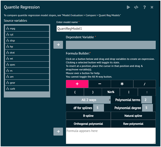
Quantile Regression
This function fits a quantile regression model, which models a desired quantile (i.e. percentile) of the outcome variable. A typical quantile to model is 0.5, i.e. the median. A model summary and parameter estimates with 95% confidence intervals are provided.
To analyse it in BioStat Prime user must follow the steps as given.
- Steps
Load the dataset -> Click on the Model Fitting tab in main menu -> Select Regression -> This leads to analysis techniques, choose Quantile Regression -> There will appear a dialog -> Select the model name, dependent variables, estimation method, standard error method and populate the formula builder in the dialog -> Finally execute the plot and visualise the output in output window.

Attributes
- Enter Model Name
the desired name of the model
- Dependent Variable
Specify the dependent variable for the model. The desired quantile of this variable will be modeled. This must be numeric.
- Formula Builder
Specify the model terms using formula notation. Numeric, factor, ordered factor, and character variables are allowed. Character variables will be coerced to factors.
- Quantile (0-1)
Specify the desired quantile to model for the dependent variable. 0.5 (the median) is the default and is a typical quantity.
- Estimation Method
Specify the estimation method for the model parameters. The Barrodale and Roberts method is the default and is efficient for models with several thousand observations. The Frisch-Newton and the Frisch-Newton, preprocessing approach might be advantageous for large and very large problems, respectively, especially in cases with a small number of estimated parameters. For large sample sizes with a large number of parameters, the Frisch-Newton, sparse method may be needed. See the references in the R Help for details.
- Standard Error Method
Specify the method used to estimate standard errors and confidence intervals. The Rank method provides confidence intervals only, can be slow to run for larger sample sizes (n > 1000), and is based on inverting a rank test. The IID method assumes the errors are independent and identically distributed (iid). The NID method presumes local linearity in the quantile and computes a sandwich estimate using a local estimate of sparsity. The Kernal method uses a kernal estimate of the sandwich. The Bootstrap method uses a re-sampling bootstrap approach to estimate the standard errors. See the references in the R Help for details.
- Bootstrap Samples
Desired number of bootstrap samples for the bootstrap standard error approach. The default is 2000 samples.