Distribution Analysis

Anderson-Darling Normality Test

The Anderson-Darling test is one such test, and it is specifically used for testing the goodness of fit of a sample to a specified distribution, often the normal distribution.

To analyse it in BioStat Prime user must follow the steps as given.

Style

Load the dataset -> Click on the analysis tab in main menu -> Select Distribution tab -> The Distribution tab contains 7 options, select the first one namely Anderson-Darling Normality test -> This leads to analysis technique in the dialog -> Select variables to target -> Execute the dialog.

Kolmogorov-Smirnov Normality Test

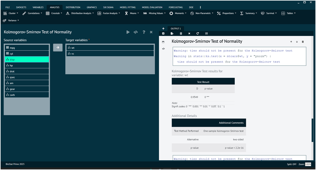
The Kolmogorov-Smirnov (K-S) test for normality is a non-parametric test used to determine whether a sample comes from a normal distribution. It is based on the cumulative distribution function (CDF) of the normal distribution and involves comparing the observed cumulative distribution of the data with the expected cumulative distribution of a normal distribution.

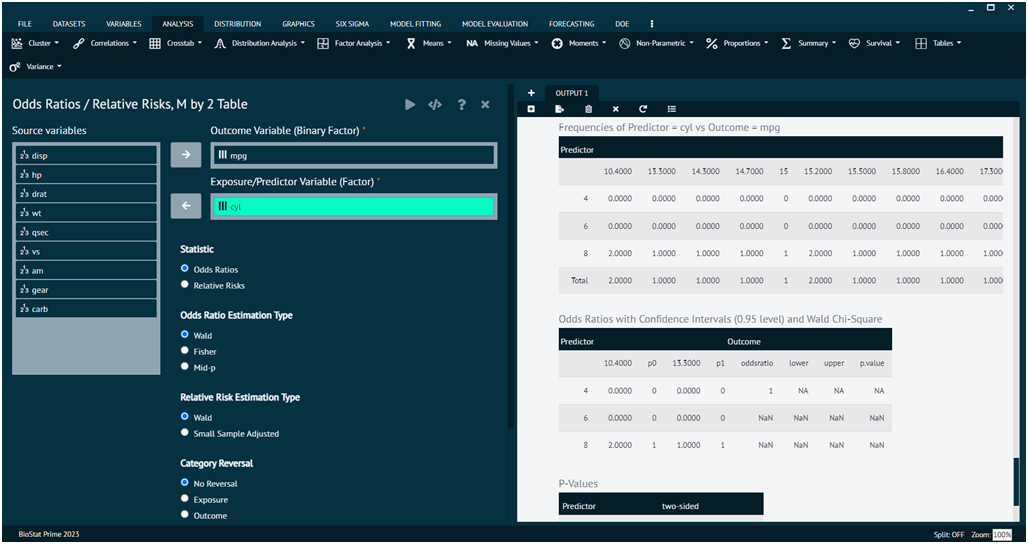
To analyse it in BioStat Prime user must follow the steps as given.

Steps

Load the dataset -> Click on the analysis tab in main menu select Distribution tab -> The Distribution tab contains 7 options, select the second one namely Kolmogorov-Smirnov Normality test -> This leads to analysis technique in the dialog -> Select variables to target -> Execute the dialog.

Shapiro-Wilk Normality Test

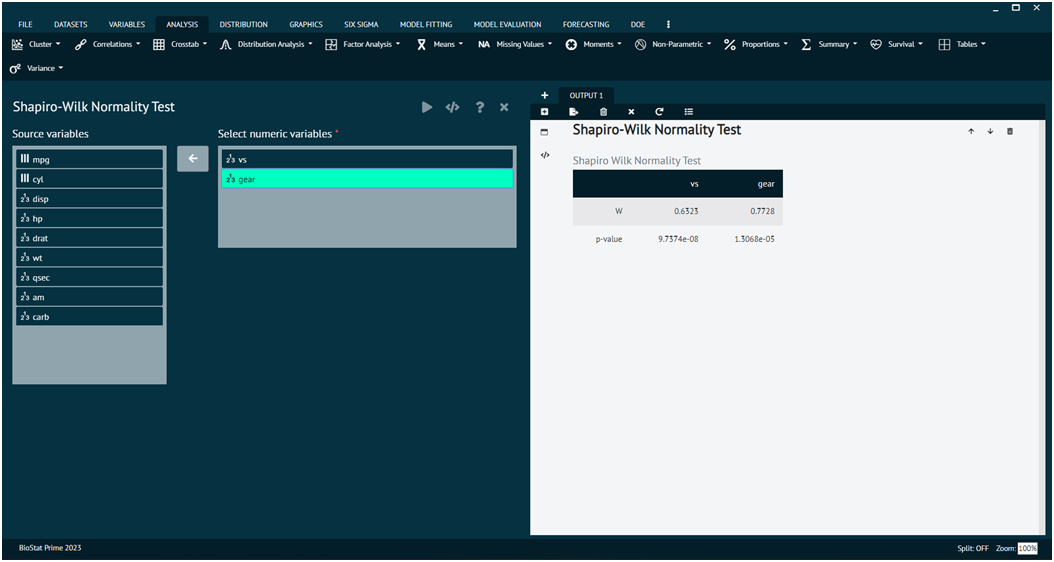
The Shapiro-Wilk test is a statistical test used to assess whether a sample comes from a normally distributed population. It is commonly used for testing the assumption of normality in statistical analyses.

To analyse it in BioStat Prime user must follow the steps as given.

Steps

Load the dataset -> Click on the analysis tab in main menu -> Select Distribution tab -> The Distribution tab contains 7 options, select the third one namely Shapiro-Wilk Normality Test -> This leads to the analysis technique in the dialog -> Select variables to target -> Execute the dialog.

Distribution Fit

Distribution fitting is a statistical technique used to model and describe the distribution of a dataset by finding the probability distribution that best fits the observed data.

To analyse it in BioStat Prime user must follow the steps as given.

Step

Load the dataset -> Click on the analysis tab in main menu -> Select Distribution tab -> The Distribution tab contains 7 options, select the fifth one namely Distribution Fit -> This leads to the analysis technique in the dialog -> Select variables to target -> Fit the test for various distributions -> Execute the dialog.

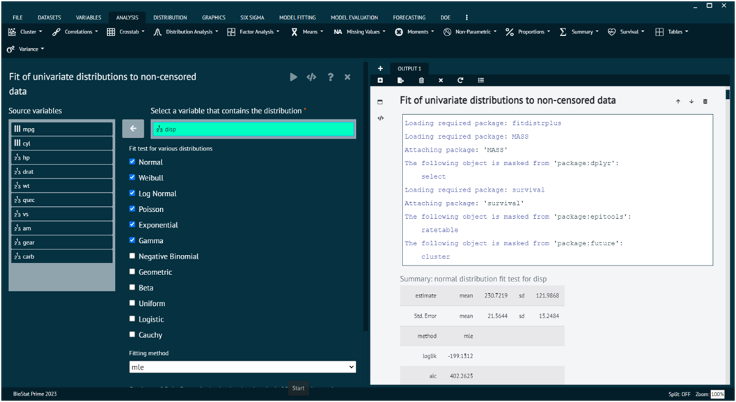
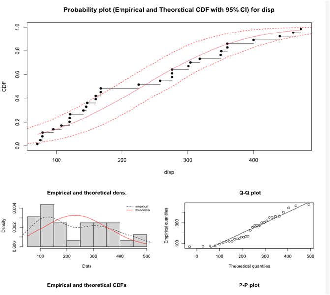
The various distributions are visible in the output window.

The four possible fitting methods are described below:

mle

When method="mle" (default) Maximum likelihood estimation consists in maximizing the log-likelihood. A numerical optimization is carried out in mledist via optim to find the best values (see mledist for details).

mme

When method="mme" Moment matching estimation consists in equalizing theoretical and empirical moments. Estimated values of the distribution parameters are computed by a closed-form formula for the following distributions : "norm", "lnorm", "pois", "exp", "gamma", "nbinom", "geom", "beta", "unif" and "logis". Otherwise the theoretical and the empirical moments are matched numerically, by minimization of the sum of squared differences between observed and theoretical moments. In this last case, further arguments are needed in the call to fitdist: order and memp (see mmedist for details).

qme

When method = "qme" Quantile matching estimation consists in equalizing theoretical and empirical quantile. A numerical optimization is carried out in qmedist via optim to minimize of the sum of squared differences between observed and theoretical quantiles. The use of this method requires an additional argument probs, defined as the numeric vector of the probabilities for which the quantile(s) is(are) to be matched (see qmedist for details).

mge

When method = "mge" Maximum goodness-of-fit estimation consists in maximizing a goodness-of-fit statistics. A numerical optimization is carried out in mgedist via optim to minimize the goodness-of-fit distance. The use of this method requires an additional argument gof coding for the goodness-of-fit distance chosen. One can use the classical Cramer-von Mises distance ("CvM"), the classical Kolmogorov-Smirnov distance ("KS"), the classical Anderson-Darling distance ("AD") which gives more weight to the tails of the distribution, or one of the variants of this last distance proposed by Luceno (2006) (see mgedist for more details). This method is not suitable for discrete distributions.

mse

When method = "mse" Maximum goodness-of-fit estimation consists in maximizing the average log spacing. A numerical optimization is carried out in msedist via optim.

Statistics of importance are Cramer-von Mises, Anderson-Darling and Kolmogorov statistics for continuous distributions and Chi-squared statistics for discrete ones ( "binom", "nbinom", "geom", "hyper" and "pois" )

Distribution Fit with Gamlss

The Gamlss package in R is used for fitting Generalized Additive Models for Location, Scale, and Shape (GAMLSS).

GAMLSS is a flexible framework for modeling distributions and is capable of handling a wide range of distributional shapes.

BioStat Prime utilizes this package of R to aids user to fit different parametric gamlss.family distributions from R pkg gamlss.

To analyse it in BioStat Prime user must follow the steps as given.

Steps

Load the dataset -> Click on the analysis tab in main menu -> Select Distribution tab -> The Distribution tab contains 7 options, select the sixth one namely Distribution Fit with Gamlss -> This leads to the analysis technique in the dialog -> Select variables that contains distribution -> Check the options at the bottom as per the preference -> Execute the dialog.

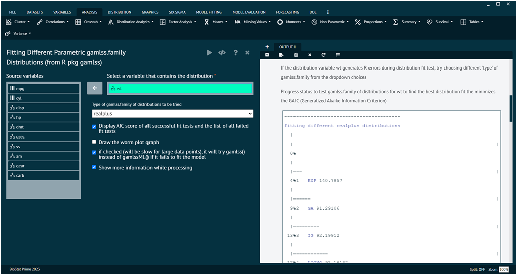
The function fitDist() is using the function gamlssML() to fit all relevant parametric gamlss.family distributions, specified by the argument type, to a single data vector (with no explanatory variables). The final marginal distribution is the one selected by the generalised Akaike information criterion with penalty k. The default is k=2 i.e AIC which means that the "best" distribution is selected according to the classic AIC. k can be set to anything, such as log(n) for the BIC (not provided on the dialog at this time)

The following are the different type argument:

realAll

All the gamlss.family (not provided on the dialog at this time) continuous distributions defined on the real line, i.e. realline and the real positive line i.e. realplus

realline

The gamlss.family continuous distributions : "NO", "GU", "RG" ,"LO", "NET", "TF", "TF2", "PE","PE2", "SN1", "SN2", "exGAUS", "SHASH", "SHASHo","SHASHo2", "EGB2", "JSU", "JSUo", "SEP1", "SEP2", "SEP3", "SEP4", "ST1", "ST2", "ST3", "ST4", "ST5", "SST", "GT"

realplus

The gamlss.family continuous distributions in the positive real line: "EXP", "GA","IG","LOGNO", "LOGNO2","WEI", "WEI2", "WEI3", "IGAMMA","PARETO2", "PARETO2o", "GP", "BCCG", "BCCGo", "exGAUS", "GG", "GIG", "LNO","BCTo", "BCT", "BCPEo", "BCPE", "GB2"

real0to1

The gamlss.family continuous distributions from 0 to 1: "BE", "BEo", "BEINF0", "BEINF1", "BEOI", "BEZI", "BEINF", "GB1""

counts

The gamlss.family distributions for counts: "PO", "GEOM", "GEOMo","LG", "YULE", "ZIPF", "WARING", "GPO", "DPO", "BNB", "NBF","NBI", "NBII", "PIG", "ZIP","ZIP2", "ZAP", "ZALG", "DEL", "ZAZIPF", "SI", "SICHEL","ZANBI", "ZAPIG", "ZINBI", "ZIPIG", "ZINBF", "ZABNB", "ZASICHEL", "ZINBF", "ZIBNB", "ZISICHEL"

binom

The gamlss.family distributions for binomial type data :"BI", "BB", "DB", "ZIBI", "ZIBB", "ZABI", "ZABB"

Distribution Analysis Cullen and Frey Graph

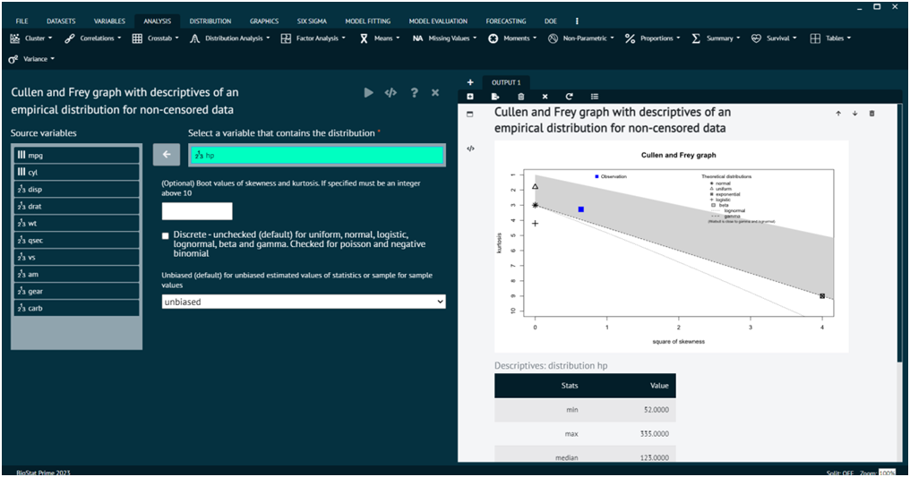
The Cullen and Frey graph, also known as the Cullen and Frey graph for skewness and kurtosis, is a graphical method for assessing the skewness and kurtosis of a dataset. It's a visual tool that helps you quickly inspect the departure from normality in terms of skewness and kurtosis.

BioStat Prime aids users to derive Cullen and frey graph with descriptive of an empirical distribution of a non-censored data.

To analyse it in BioStat Prime user must follow the steps as given.

Steps

Load the dataset -> Click on the analysis tab in main menu -> Select Distribution tab -> The Distribution tab contains 7 options, select the seventh one namely Distribution Analysis Cullen and Frey Graph -> This leads to the analysis technique in the dialog -> Select variables that contains distribution -> Check the options at the bottom as per the preference -> Execute the dialog.